The effects of Brexit#

The aim of this notebook is to estimate the causal impact of Brexit upon the UK’s GDP. This will be done using the synthetic control approach. As such, it is similar to the policy brief “What can we know about the cost of Brexit so far?” [Springford, 2022] from the Center for European Reform. That approach did not use Bayesian estimation methods however.

I did not use the GDP data from the above report however as it had been scaled in some way that was hard for me to understand how it related to the absolute GDP figures. Instead, GDP data was obtained courtesy of Prof. Dooruj Rambaccussing. Raw data is in units of trillions of USD.

import arviz as az
import matplotlib.pyplot as plt
import numpy as np
import pandas as pd
import seaborn as sns
from pymc_extras.prior import Prior

import causalpy as cp

%load_ext autoreload
%autoreload 2
%config InlineBackend.figure_format = 'retina'
seed = 42

Load data#

df = (
    cp.load_data("brexit")
    .assign(Time=lambda x: pd.to_datetime(x["Time"]))
    .set_index("Time")
    .loc[lambda x: x.index >= "2009-01-01"]
    # manual exclusion of some countries
    .drop(["Japan", "Italy", "US", "Spain", "Portugal"], axis=1)
)

# specify date of the Brexit vote announcement
treatment_time = pd.to_datetime("2016 June 24")

df.head()

	Australia	Austria	Belgium	Canada	Denmark	Finland	France	Germany	Iceland	Luxemburg	Netherlands	New_Zealand	Norway	Sweden	Switzerland	UK
Time
2009-01-01	3.84048	0.802836	0.94117	16.93824	4.50096	0.51052	5.05450	6.63471	5.18157	0.114836	1.634391	0.47336	7.78753	10.32220	1.476532	4.61881
2009-04-01	3.86954	0.796545	0.94162	16.75340	4.41372	0.50829	5.05375	6.64530	5.16171	0.116259	1.634432	0.47916	7.71903	10.32867	1.485509	4.60431
2009-07-01	3.88115	0.799937	0.95352	16.82878	4.42898	0.51299	5.06237	6.68237	5.24132	0.118747	1.640982	0.48188	7.72400	10.32328	1.502506	4.60722
2009-10-01	3.91028	0.803823	0.96117	17.02503	4.43300	0.50903	5.09832	6.73155	5.22482	0.119302	1.650866	0.48805	7.72812	10.37107	1.515139	4.62152
2010-01-01	3.92716	0.800510	0.96615	17.23041	4.47128	0.51413	5.11625	6.78621	4.91128	0.121414	1.647748	0.49349	7.87891	10.64833	1.525864	4.65380

# get useful country lists
target_country = "UK"
all_countries = df.columns
other_countries = all_countries.difference({target_country})
all_countries = list(all_countries)
other_countries = list(other_countries)

Data visualization#

az.style.use("arviz-white")

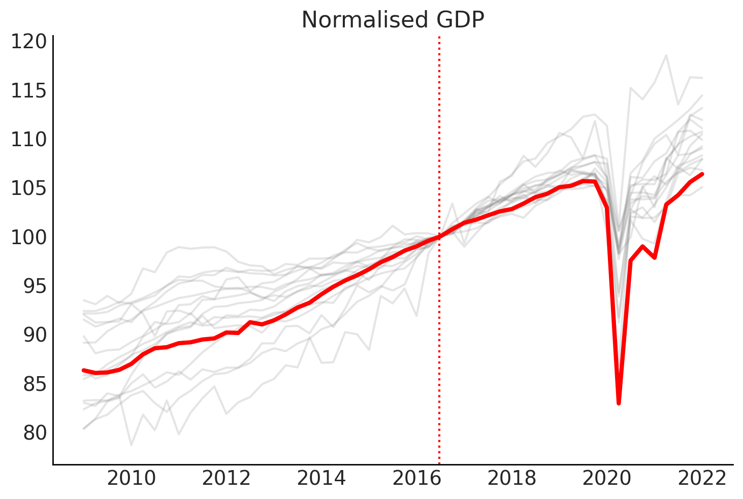
# Plot the time series normalised so that intervention point (Q3 2016) is equal to 100
gdp_at_intervention = df.loc[pd.to_datetime("2016 July 01"), :]
df_normalised = (df / gdp_at_intervention) * 100.0

# plot
fig, ax = plt.subplots()
for col in other_countries:
    ax.plot(df_normalised.index, df_normalised[col], color="grey", alpha=0.2)

ax.plot(df_normalised.index, df_normalised[target_country], color="red", lw=3)
# ax = df_normalised.plot(legend=False)

# formatting
ax.set(title="Normalised GDP")
ax.axvline(x=treatment_time, color="r", ls=":");

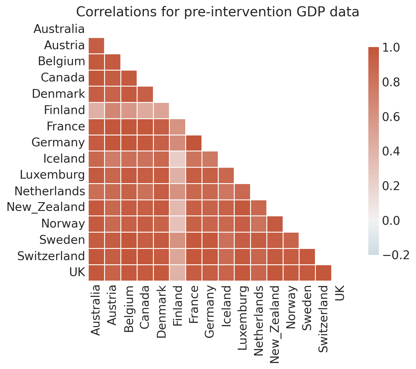
../_images/d913d116d1a335951d4f191164078e8959df7c2ea9d2464594c8655dde083b96.png

# Examine how correlated the pre-intervention time series are

pre_intervention_data = df.loc[df.index < treatment_time, :]

corr = pre_intervention_data.corr()

f, ax = plt.subplots(figsize=(8, 6))
ax = sns.heatmap(
    corr,
    mask=np.triu(np.ones_like(corr, dtype=bool)),
    cmap=sns.diverging_palette(230, 20, as_cmap=True),
    vmin=-0.2,
    vmax=1.0,
    center=0,
    square=True,
    linewidths=0.5,
    cbar_kws={"shrink": 0.8},
)
ax.set(title="Correlations for pre-intervention GDP data");

../_images/8aafe77496f5293e5f17c3c035cd37376b46ae4f01f0a71e257f27ceaf61bdf7.png

Run the analysis#

Note: The analysis is (and should be) run on the raw GDP data. We do not use the normalised data shown above which was just for ease of visualization.

Note

The random_seed keyword argument for the PyMC sampler is not necessary. We use it here so that the results are reproducible.

sample_kwargs = {"tune": 1000, "target_accept": 0.99, "random_seed": seed}

result = cp.SyntheticControl(
    df,
    treatment_time,
    control_units=other_countries,
    treated_units=[target_country],
    model=cp.pymc_models.WeightedSumFitter(
        sample_kwargs=sample_kwargs,
    ),
)

Initializing NUTS using jitter+adapt_diag...
Multiprocess sampling (4 chains in 4 jobs)
NUTS: [beta, y_hat_sigma]

Sampling 4 chains for 1_000 tune and 1_000 draw iterations (4_000 + 4_000 draws total) took 70 seconds.
There were 1 divergences after tuning. Increase `target_accept` or reparameterize.
Chain 0 reached the maximum tree depth. Increase `max_treedepth`, increase `target_accept` or reparameterize.
Chain 1 reached the maximum tree depth. Increase `max_treedepth`, increase `target_accept` or reparameterize.
Chain 2 reached the maximum tree depth. Increase `max_treedepth`, increase `target_accept` or reparameterize.
Chain 3 reached the maximum tree depth. Increase `max_treedepth`, increase `target_accept` or reparameterize.
The rhat statistic is larger than 1.01 for some parameters. This indicates problems during sampling. See https://arxiv.org/abs/1903.08008 for details
Sampling: [beta, y_hat, y_hat_sigma]
Sampling: [y_hat]
Sampling: [y_hat]
Sampling: [y_hat]
Sampling: [y_hat]

While we are at it, let’s plot the graphviz representation of the model. This shows us the inner workings of the WeightedSumFitter class which defines our synthetic control model with a sum to 1 constraint on the donor weights (here labelled as coeffs). This will be particularly useful when we come to exploring custom priors (see below).

result.model.to_graphviz()

../_images/61c8a8681a93fe50344da65bc7a5c9e62f0f1272ffe438d1f8a1ce0de790d264.svg

We currently get some divergences, but these are mostly dealt with by increasing tune and target_accept sampling parameters. Nevertheless, the sampling of this dataset/model combination feels a little brittle.

result.idata

arviz.InferenceData

posterior
posterior_predictive
sample_stats
prior
prior_predictive
observed_data
constant_data

Check the MCMC chain mixing via the Rhat statistic.

az.summary(result.idata, var_names=["~mu"])

	mean	sd	hdi_3%	hdi_97%	mcse_mean	mcse_sd	ess_bulk	ess_tail	r_hat
beta[UK, Australia]	0.121	0.074	0.001	0.243	0.003	0.001	607.0	656.0	1.00
beta[UK, Austria]	0.046	0.042	0.000	0.123	0.001	0.001	808.0	703.0	1.01
beta[UK, Belgium]	0.052	0.048	0.000	0.140	0.001	0.001	784.0	618.0	1.00
beta[UK, Canada]	0.038	0.023	0.000	0.077	0.001	0.000	472.0	476.0	1.01
beta[UK, Denmark]	0.085	0.065	0.000	0.200	0.002	0.001	581.0	573.0	1.00
beta[UK, Finland]	0.041	0.039	0.000	0.113	0.001	0.001	873.0	935.0	1.00
beta[UK, France]	0.031	0.028	0.000	0.084	0.001	0.001	749.0	728.0	1.00
beta[UK, Germany]	0.026	0.025	0.000	0.072	0.001	0.001	680.0	897.0	1.00
beta[UK, Iceland]	0.154	0.041	0.075	0.230	0.001	0.001	844.0	943.0	1.00
beta[UK, Luxemburg]	0.049	0.045	0.000	0.134	0.001	0.001	738.0	553.0	1.00
beta[UK, Netherlands]	0.048	0.043	0.000	0.126	0.001	0.001	996.0	995.0	1.00
beta[UK, New_Zealand]	0.062	0.055	0.000	0.164	0.002	0.001	627.0	605.0	1.00
beta[UK, Norway]	0.082	0.045	0.000	0.156	0.002	0.001	621.0	568.0	1.01
beta[UK, Sweden]	0.100	0.031	0.043	0.160	0.001	0.001	837.0	719.0	1.01
beta[UK, Switzerland]	0.065	0.057	0.000	0.172	0.001	0.001	3963.0	2199.0	1.00
y_hat_sigma[UK]	0.031	0.005	0.023	0.040	0.000	0.000	1036.0	1488.0	1.00

You can inspect the traces in more detail with:

az.plot_trace(result.idata, var_names="~mu", compact=False);

az.style.use("arviz-darkgrid")

fig, ax = result.plot(plot_predictors=False)

for i in [0, 1, 2]:
    ax[i].set(ylabel="Trillion USD")

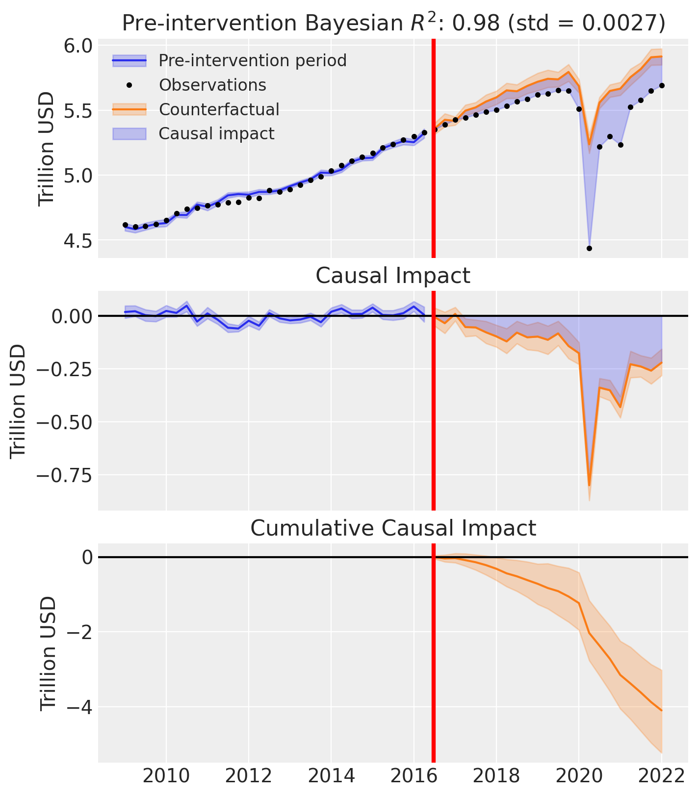
../_images/19d41d820157994b7ab17b9974de02be1f9b22dbc1a5074701719eb1af08d8da.png

result.summary()

================================SyntheticControl================================
Control units: ['Australia', 'Austria', 'Belgium', 'Canada', 'Denmark', 'Finland', 'France', 'Germany', 'Iceland', 'Luxemburg', 'Netherlands', 'New_Zealand', 'Norway', 'Sweden', 'Switzerland']
Treated unit: UK
Model coefficients:
    Australia    0.12, 94% HDI [0.0086, 0.27]
    Austria      0.046, 94% HDI [0.0013, 0.15]
    Belgium      0.052, 94% HDI [0.0016, 0.17]
    Canada       0.038, 94% HDI [0.0025, 0.085]
    Denmark      0.085, 94% HDI [0.0031, 0.23]
    Finland      0.041, 94% HDI [0.0015, 0.14]
    France       0.031, 94% HDI [0.0011, 0.1]
    Germany      0.026, 94% HDI [0.00096, 0.086]
    Iceland      0.15, 94% HDI [0.075, 0.23]
    Luxemburg    0.049, 94% HDI [0.0011, 0.16]
    Netherlands  0.048, 94% HDI [0.0021, 0.16]
    New_Zealand  0.062, 94% HDI [0.0015, 0.19]
    Norway       0.082, 94% HDI [0.0076, 0.17]
    Sweden       0.1, 94% HDI [0.039, 0.16]
    Switzerland  0.065, 94% HDI [0.0024, 0.2]
    y_hat_sigma  0.031, 94% HDI [0.023, 0.041]

Effect Summary Reporting#

For decision-making, you often need a concise summary of the causal effect with key statistics. The effect_summary() method provides a decision-ready report with average and cumulative effects, HDI intervals, tail probabilities, and relative effects. This provides a comprehensive summary without manual post-processing.

# Generate effect summary for the full post-period
stats = result.effect_summary()
stats.table

	mean	median	hdi_lower	hdi_upper	p_gt_0	relative_mean	relative_hdi_lower	relative_hdi_upper
average	-0.178323	-0.179121	-0.227586	-0.127143	0.0	-3.164222	-4.005843	-2.278178
cumulative	-4.101438	-4.119792	-5.234484	-2.924293	0.0	-3.164222	-4.005843	-2.278178

# View the prose summary
print(stats.text)

Post-period (2016-07-01 00:00:00 to 2022-01-01 00:00:00), the average effect was -0.18 (95% HDI [-0.23, -0.13]), with a posterior probability of an increase of 0.000. The cumulative effect was -4.10 (95% HDI [-5.23, -2.92]); probability of an increase 0.000. Relative to the counterfactual, this equals -3.16% on average (95% HDI [-4.01%, -2.28%]).

# You can also analyze a specific time window, e.g., the first year after Brexit
stats_window = result.effect_summary(
    window=(pd.to_datetime("2016-06-24"), pd.to_datetime("2017-06-24"))
)
stats_window.table

	mean	median	hdi_lower	hdi_upper	p_gt_0	relative_mean	relative_hdi_lower	relative_hdi_upper
average	-0.021407	-0.021822	-0.064357	0.021860	0.1635	-0.393064	-1.17724	0.406281
cumulative	-0.085627	-0.087289	-0.257429	0.087441	0.1635	-0.393064	-1.17724	0.406281

Custom priors#

The analysis above is all based upon the default priors for the WeightedSumFitter class. But this might not always be appropriate. In particular the default Priors are Dirichlet distributed with an alpha parameter of 1. This corresponds to a uniform prior over the simplex.

But we might have different prior beliefs. For example, we might think that some control units will play a larger role and some control units will be irrelevant. In which case, we could use as less concentrated prior, such as \(\mathrm{Dirichlet}(0.1)\).

We can do this in the code below.

n_control_units = len(other_countries)

result_custom = cp.SyntheticControl(
    df,
    treatment_time,
    control_units=other_countries,
    treated_units=[target_country],
    model=cp.pymc_models.WeightedSumFitter(
        sample_kwargs=sample_kwargs,
        priors={
            "beta": Prior(
                "Dirichlet",
                a=0.1 * np.ones(n_control_units),
                dims=["treated_units", "coeffs"],
            ),
        },
    ),
)

Initializing NUTS using jitter+adapt_diag...
Multiprocess sampling (4 chains in 4 jobs)
NUTS: [beta, y_hat_sigma]

Sampling 4 chains for 1_000 tune and 1_000 draw iterations (4_000 + 4_000 draws total) took 81 seconds.
There were 168 divergences after tuning. Increase `target_accept` or reparameterize.
Chain 0 reached the maximum tree depth. Increase `max_treedepth`, increase `target_accept` or reparameterize.
Chain 1 reached the maximum tree depth. Increase `max_treedepth`, increase `target_accept` or reparameterize.
Chain 2 reached the maximum tree depth. Increase `max_treedepth`, increase `target_accept` or reparameterize.
Chain 3 reached the maximum tree depth. Increase `max_treedepth`, increase `target_accept` or reparameterize.
The rhat statistic is larger than 1.01 for some parameters. This indicates problems during sampling. See https://arxiv.org/abs/1903.08008 for details
The effective sample size per chain is smaller than 100 for some parameters.  A higher number is needed for reliable rhat and ess computation. See https://arxiv.org/abs/1903.08008 for details
Sampling: [beta, y_hat, y_hat_sigma]
Sampling: [y_hat]
Sampling: [y_hat]
Sampling: [y_hat]
Sampling: [y_hat]

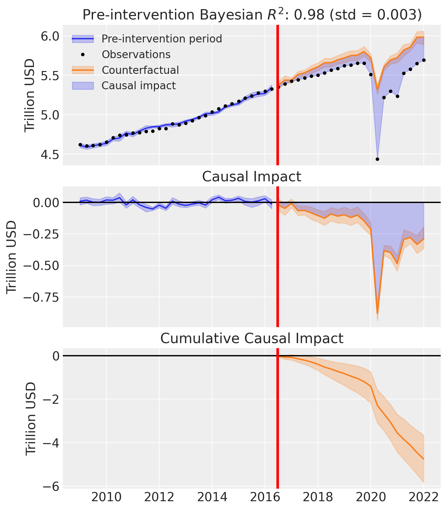
The main results plot shows only minor differences in terms of fitting.

fig, ax = result_custom.plot(plot_predictors=False)

for i in [0, 1, 2]:
    ax[i].set(ylabel="Trillion USD")

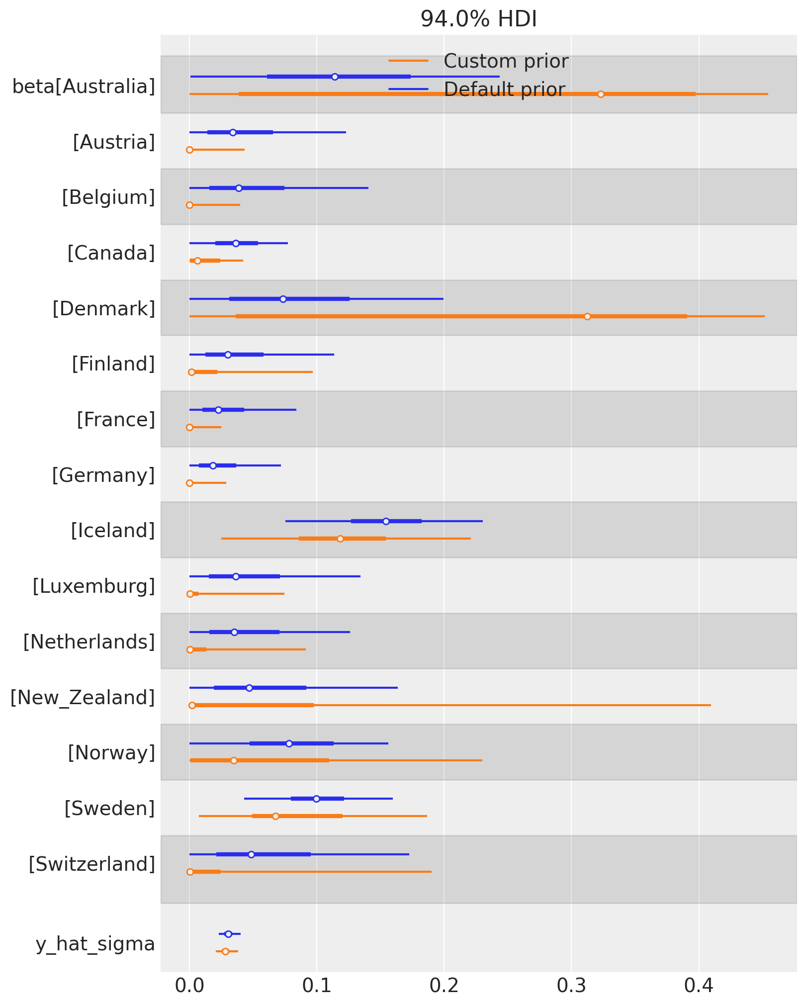
../_images/00a64132dfc94ffa5b402526b797b4f52a6a7809692eeab93f6737b8cc35d504.png

We can also examine the effect of changing the Dirichlet prior on the posterior distribution of weights. TWe can see that the custom prior of \(\mathrm{Dirichlet}(0.1)\) results in more sparse weights over control countries. The posterior of many countries are more concentrated near zero (e.g. Austria, Canada, Germany, etc), while others have increased in importance (e.g. Denmark, and Australia).

This is a rich area for discussion, but the key point is that users can define their own prior beliefs about the weights in the synthetic control model. There are some benefits from having ‘sparsifying’ priors in that they can help identify a smaller set of key control units that are most relevant to constructing the synthetic control.

../_images/f56e77d65f0ad776527e1c80346b53ffeb438b8e601bb6e5e2cf760ad6619783.png

References#

[1]

John Springford. What can we know about the cost of brexit so far? 2022. URL: https://www.cer.eu/publications/archive/policy-brief/2022/cost-brexit-so-far.